
Return to MODULE PAGE
Connectionism: An Introduction (page 2)
Rob Stufflebeam: Designer, Programmer & Author
Unit behavior
As you discovered in the previous lesson, connectionist models are based on how information processing occurs in biological neural networks. Consequently, a unit in a connectionist network is analogous to a neuron. A connection in a connectionist model is analogous to a synapse. So, just as neurons are the basic information processing structures in biological neural networks, units are the basic information processing structures in connectionist networks. And just as synapses are conduits through which information flows from one neuron to another, connections are conduits through which information flows from one unit to another. The aim of this lesson is to introuduce you to the nature of the information processing (computation) that occurs within a unit.
Units as computers
In general functional terms, a unit in a connectionist network does very much the same thing a neuron does in a biological neural network. Namely, it receives INPUT "signals" from other units, it computes an OUTPUT "signal" based on its INPUT, then it sends that OUTPUT to other units. Let's think about that for a moment. It has been noted elsewhere (see Functionalism) that the following animation captures the one feature all computers have in common.
What is that feature? Well, that every computer has three
functional components:
(1) INPUT information,
(2) OUTPUT information, and
(3) a computational process whereby the INPUT determines the OUTPUT.
Just as each neuron in a neural network has these components, so too does each unit in a connectionist network. Thus, not only is it apporpriate to say of a neural network that it is a computer, it is appropriate to describe each of the network's basic processing units as computers too. For this reason, what follows is your introduction to how computation (information processing) occurs within the most basic of computers in a connectionist network -- the unit.
Activations
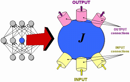
The following image represents a typical (hidden) unit in a connectionist network. Since it would be awkward to keep saying "the unit," let's call this unit 'J'. The image (below) on the left shows that J is connected to each of the units in the layers below it and above it. The image in the right captures J in all its anatomical detail. In general functional terms, J does very much the same thing a neuron does in a biological neural network. Namely, it receives INPUT "signals" from other units, it computes an OUTPUT signal based on its INPUT, then it sends its OUTPUT "signal" to other units. J receives INPUT via the connections represented in yellow. J sends OUTPUT via the connections represented in pink.
The "signals" J receives as INPUT and sends as OUTPUT are called activation values (or simply activations). As the term 'value' suggests, activations in connectionist networks are always numbers. Always. What do these numbers represent? Because units in a connectionist network are analogous to neurons in biological neural networks, are activation values analogous to neural signals (action potentials)?
Yes and no. Although neurons can be construed as feature detectors and units in some connectionist networks are designed to behave like feature detectors (see McCulloch-Pitts Neurons), units in most connectionist models are not designed to send discrete (digital) "on" or "off" signals. Hence, in most connectionist models, activation values are never 1 (for "on" or "the feature is present") or 0 (for "off" or "the feature is not present"). Instead, in most connectionist models, activation values are analogous to a neuron's firing rate or how "actively" it is sending "signals" to other neurons. Between being the least active a neuron can be and the most active it can be, there is quite a bit of variability. The same is true of units. In a connectionist network, this variability is captured by a numerical value within a predetermined range, usually 0 to 1. A unit with an activation value of 0 would be analogous to a neuron that is the least active it could be. A unit with an activation of 1 would be analogous to a neuron that is the most active it could be. Units in most connectionist networks must have an activation value between 0 and 1 -- for example, .1, .35, .67, .8, etc. Such nondiscrete (analog) values are comparable to a neuron's level of activity somewhere between being the least active or most active it could be. Such values could also be construed as a measure of how probable a particular feature is present, but let's ignore this. Hence, consider a unit's activation value to be analogous to a neuron's firing rate.
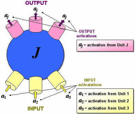
The INPUT signals J receives from other units (via its INPUT connections) are its INPUT activations. Because J has three INPUT connections, at any given moment it will receive three INPUT activations. These are represented by the symbols a1, a2, and a3. The OUTPUT signals J sends to other units (via its OUTPUT connections) are its OUTPUT activations. Regardless of what that value is at any moment, say, .7, J will send the same value through each of its OUTPUT connections. Accordingly, J's OUTPUT activation is represented by a single symbol -- aj.
Connection weights
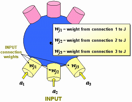
Although it is true that units compute their activation value (OUTPUT) on the basis of their INPUT activations, the INPUT activations to a unit are not the only values it needs to "know" before it can compute its OUTPUT activation. It also needs to "know" how strongly or weakly an INPUT activation should affect its behavior. In much the same way that criticism from someone not strongly connected to you will have little affect on your behavior, a high INPUT activation sent through a weak connection will not much affect J's behavior. The strength or weakness of a connection is measured by a connection weight. In the image below, the symbols wj1, wj2, and wj3 represent the connection weights between J and its INPUT units.
As is the case with activation values, connection weights are usually nondiscrete values between a certain range, usually -1 to 1. A low connection weight (say, -.8) represents a weak connection. A high connection weight (e.g., .7) represents a strong connection. Connection weights are analogous to an important aspect of biological neural networks; namely, that synapses are either inhibitory or excitatory. Inhibitory connections reduce a neuron's level of activity; excitatory connections increase it.
How does a unit compute its OUTPUT?
Combined INPUT
But just as no one neuron's behavior is determined by a single synapse, the behavior of J is never determined by an INPUT signal sent via a single connection, however strong or weak that connection might be. So, just as a neuron's behavior is determined by its COMBINED INPUT, which is the sum of its total inhibitory and excitatory INPUT signals, J's behavior (activation) depends on its COMBINED INPUT. The COMBINED INPUT to J (cj) is the sum of each INPUT activation multiplied by its connection weight. Computing the COMBINED INPUT is the first part of the information processing occurring within J. A mathematical description of this part of the processing is represented below:
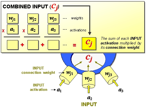
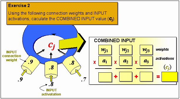
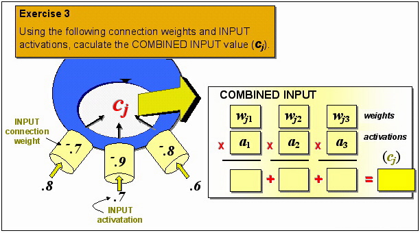
The ellipses ('. . .') in the above diagram indicate that if a unit has more than three INPUT connections (or fewer for that matter), its combined INPUT will be the sum of each INPUT activation multiplied by its connection weight. After all, units in some connectionist networks have more than (or fewer than) three INPUT connections. But J has only three. Before learning what else is required before J can compute its OUTPUT, what follows are three exercises for you to practice this part of the computation occurring within J.

Activation function
In a biological neural network, a neuron will "fire" only when its COMBINED INPUT value is equal to or exceeds its threshold. And when it fires, its signal is (almost) always of the same magnitude or strength. Hence, a very high (excitatory) COMBINED INPUT will NOT result in a neuron sending a very strong neural signal. A very low (inhibitory) COMBINED INPUT will not result in a neuron sending a very weak signal. A neural signal is neural signal. What varies is how often they occur, not their strength. All things being equal, neurons are not susceptible to "power surges."
The same holds for units in a connectionist model. But since the OUTPUT activation of a unit represents how active it is, NOT the strength of its "signal," the OUTPUT activation of a unit and the OUTPUT signal of a neuron are not entirely analogous. Nevertheless, just as a neuron cannot exceed its usual signal strength, it cannot exceed its maximum or minimum rates of fire either. So, because a unit's activation value is analogous to a neuron's firing rate, the OUTPUT activation of a unit can NEVER exceed its maximum or minimum activation values. For J, these values are 1 and 0 respectively. Hence, a very high COMBINED INPUT of 2.01 (see Exercise 2 above) will NOT result in an activation value greater than 1. And a COMBINED INPUT of -1.67 (see Exercise 3 above) will NOT result in an activation value lower than 0.
To ensure that the OUTPUT activation of a unit NEVER exceeds its maximum or minimum activation values, a unit's COMBINED INPUT must be put through an activation function. An activation function is simply a mathematical formula that "squashes" the COMBINED INPUT into the activation value range, which for us is 0 to 1. Hence, when the COMBINED INPUT to J is put through its activation function, the result is J's OUTPUT activation. (There are many activation functions used in connectionist networks, the most common of which is the sigmoid function. Don't worry about the math. It is the mapping activation function that you need to understand.) This completes the second part of the INPUT-to-OUTPUT information processing occurring within J. A description (and animation) of this part of the processing is represented below.
The following figure summarize the computation occurring within a typical unit. The right portion captures the flow of information. The left portion captures the steps in the computation.
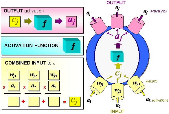
Since J's OUTPUT becomes the INPUT activation to each of the units to which it is connected, the cycle of INPUT-to-OUTPUT information processing just described is then repeated within each of the units in the layer above J.
This completes the lesson on unit behavior. We now turn our attention to what networks of such units are capable of doing and how they learn.