Return to MODULE PAGE

Connectionist Networks that Can See

David Leech Anderson: Author
(An unknown undergraduate from Illinois Wesleyan from the early 2000s): Author

It is time to see a connectionist network at work. Elsewhere, you can see how a symbol-processing computer program can represent the shape of an object and recognize when two objects are the same shape and size (see Chain Codes: An Introduction). The connectionist network that you will see in action below, will do some rather impressive things that simple chaincodes could not.

There are two capabilities of our connectionist network that are of particular note. First, the connectionist network described here has the flexibility to recognize properties of a general kind, like the property of "wearing sunglasses". Remember that using our chaincodes, we could only tell if two objects had exactly the same shape and size. But as we process visual information about the world, the properties that we most frequently need to recognize are those properties that many different objects can possess, even if they are not exactly the same. (Note: Most properties are of this kind: being a dog, being a tree, being a house, etc.)

The second notable capability of a connectionist network is that the network doesn't have to be pre-programmed to recognize properties, it learns how to recognize the property through a special kind of training process. One of the problems of most symbol-processing programs is that the programmer has to anticipate every possible set of circumstances in the environment and hard-code the program to behave appropriately in every possible situation. But the real world seldom cooperates. The world is a complex and unpredictable place and it frequently throws out things that cannot be anticipated. That's why symbol-processing programs tend to be brittle and to fail in the rich complexity of real-world situations

The performance of connectionist networks, however, does not depend upon a programmer anticipating every possible situation in advance. Instead, if the network has been trained with a rich array of data from the world, it will often be able to handle new data quite adequately -- data that it would have been all put impossible to design a symbol-processing program to handle.

Meet GNNV

It is now time to see a real connectionist network doing some real work. The network we will be exploring is a 3-layer network that was originally developed at Carnegie Mellon University. However, it has been incorporated into a splendid graphical program by The Shelley Research Group at Illinois Wesleyan University. It is a Linux program called The GNU Neural Network Visualizer (or GNNV for short). GNNV provides a visual representation of the network which allows one to see the network change as it is being trained.

You will not be seeing the actual GNNV program on these web pages. It only runs on UNIX-based operating systems (like Linux). Instead, we have created some animations of the program that will run right on your browser. So you will get a good indication of how the program works. (If you have the proper operating system and want the program itself, it is available free from The Shelley Group's website.)

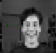GNNV uses a 3-layer network that has 960 input units (or nodes), 4 hidden units (or nodes) and 1 output node. Why are there so many (i.e., 960) input nodes? Well, this connectionist network is trained to recognize certain characteristics of peoples' faces. It "learns" how to recognize these features by analyzing data from photos that are 30 pixels by 32 pixels in size. The face at the left is one such picture. This picture is composed of 960 tiny dots (pixels) of information (30 x 32 = 960). Every pixel on the image has its own input node.

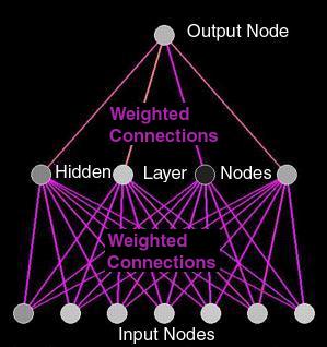It is not practical, however, to produce a visual representation of a network with 960 input nodes. Each node would have to be so small that the entire network would be one big blur. What the GNNV program does instead is to isolate sections of the network to give you a close-up view of what is going on in that particular part of the network. The program allows the viewer to pick any string of 7 input nodes to examine at a given time. Thus, the image at the right shows all 4 of the networks hidden units, it shows the output unit, but it shows only 7 of the 960 input units. You can only observe 7 at a time, but you can keep changing which 7 you observe so that with time you can see as many of the input nodes as you desire.

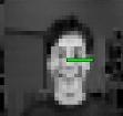The program allows the user to move a small green bar 7 pixels wide around the image to pick out the 7 input nodes to be graphically represented in the 3-layer network. In the picture at the left you can see the green bar has been positioned in the middle of the face. If you were working with the actual program, YOU would be able to choose where to locate the bar. You could leave it in one place or you could move it around. In the animations below, we will move the bar for you.

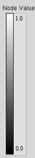As you have learned in the previous pages on connectionism, the central characteristics of a connectionist network are represented mathematically. First there is the firing rate of each unit (or node). In this program, the firing rate is represented by a number between 0 and 1. The higher the number, the higher the firing rate.

Each node is represented by a circle that can vary in shades of gray, from white all the way to black. A black unit has a very slow firing rate; a white unit has a very fast firing rate and various shades of gray represent the firiing rates in between. The bar on the right labeled "Node Value" shows the scale from 0 to 1. In the animations below, you can see some of the nodes change their firing rate, as they sometimes speed up, sometimes slow down.

A second prominent feature of a connectionist network is the role of the connection weights between the units. These connection weights are also mathematical values. Positive weights, between 0 and 1 reflect an exitatory connection. When a unit fires along an exitatory connection, a positive value is added to the combined input to that unit. Negative weights between -1 and 0 reflect an inhibatory connection. When a unit fires along an inhibatory connection, a negative value is added to the combined input to that unit, which tends to reduce the firing rate of that unit.

In the GNNV's graphical representation of the network, connections between nodes are represented with straight lines. The color of the lines reflect the connection strength between the nodes (either positive or negative). Positive weights are represented by colors from red to yellow; negative weights from medium blue to light blue. Neutral weights (around 0) will be purple.

It is now time to put all of the pieces together and observe the GNNV in action. Here you will see a session where the network is trained to "recognize" the property of "wearing sunglasses"

In the demonstration you just viewed, you watched the connectionist network go through 50 epochs or training sessions. Here is how it works.

TRAINING THE NETWORK

Training (teaching) the connectionist network happens in much the same way that a human is trained. A series of images are shown to the network for analysis and a question is asked about each of the images. If the network correctly answers the question nothing is changed. This is something like "rewarding" the network for a job well done. If the network doesn't properly answer the question it is "corrected" by changing the existing weights and nodes based on how wrong the answer was.

The whole training process is done automatically. The network is shown a picture, asked a question and then rewarded or corrected based on the answer. This process is repeated for all of the images selected. One run through the images is called an Epoch. For training purposes the network goes through 50 or more epochs to effectively train the appropriate values into the Network.

The animation above shows the change in the Neural Network over a series of 50 epochs. As one can see the resulting network has very strong connections between the first, second and fourth Hidden Nodes while the connection from the third Hidden Node is more inhibitory.

A user actually sitting at a computer with GNNV loaded onto it would also be able to see GNNV cycling through the images as it does its analysis. The images are displayed very quickly in the Image Display Window and the color of the Input Nodes, the Hidden Layer Nodes and the weights also changes depending on which image is being displayed at the time and what changes have occurred in the network's weightings from the previous epoch.

These changes in color represent the fact that GNNV is learning. Through the process, the network is being asked questions and then is being affirmed or corrected based on its answers, The changes mades to the connection weights through the training process also results in changes to the firing rates of the nodes. As a result of the entire process, it is able to more effectively recognize the appropriate pattern of information and to provide a more accurate answer to the question it is being asked.

One more demonstration

We can further see the results of training the network by selecting another set of images to analyze. The network is able to effectively recognize whether or not the people in the different image list are wearing sunglasses or not. The significance of this is that it shows that the network hasn't just "Memorized" the right answers to the images it is being shown, but rather, the network is recognizing patterns in the images that can generalize to other image sets.

Once the network has been trained the user can also click with their mouse over the Image Display Window and move the Selection Bar. The result is similar to what is shown in this animation.

As one can see in the animation above, moving the selection bar over the image displayed causes the Input Nodes to change to reflect the pixels currently under the Selection Bar. One can also seen the weights connecting the Input Nodes to the hidden layer change. The interesting thing to note here is the difference in the amount of change that occurs in the connections around the area of the image where the eyes are most often located versus other parts of the image. It is hard to see in the animation above as the change in weights is very slight when you get further down into the network. A user sitting using GNNV, however, would be able to see this association, especially if more training epochs were run.

The fact that stronger weights are tied to the Input Nodes around the eyes with less activity happening further out in the image helps to support the fact that the Neural Network has learned to recognize the difference between a person wearing sunglasses and a person not wearing sunglasses. This is because the increase in weights shows that the network knows that that is the most important part of the image to analyze for answering the question. Much like when one asks a human if another person is wearing sunglasses they don't usually stare at the person's feet to answer the question. The person, instead, knows to look at the person's face to gather the necessary information.